JCR一区 | Matlab实现1D-2D-GASF-CNN-BiLSTM-MATT的多通道输入数据分类预测
分类效果


基本介绍
Matlab实现1D-2D-GASF-CNN-BiLSTM-MATT的多通道输入数据分类预测;
数据准备:准备原始的序列数据,并将其转换为格拉姆矩阵的GASF矩阵表示。这将为每个时间步创建一个GASF图像。
2D卷积神经网络(CNN):将GASF矩阵作为输入,使用2D卷积神经网络来提取图像特征。CNN会在每个GASF图像上进行卷积和池化操作,以学习到图像中的空间模式和结构信息。这将生成一组一维向量作为CNN特征。
双向卷积神经网络(BiLSTM)和多头注意力机制:将原始鸢尾花数据输入到BiLSTM中以捕捉时间序列的依赖关系。BiLSTM将提取时间序列的特征向量。在这个过程中,还使用了多头注意力机制来融合BiLSTM的输出。最终,一组一维向量被生成作为BiLSTM特征。
特征融合:将CNN提取的特征向量和BiLSTM提取的特征向量进行融合,可以使用简单的连接操作将它们合并为一个更综合的特征向量。
全连接层和Softmax分类器:将融合的特征向量输入到全连接层中,该层可以学习到特征之间的非线性关系。最后,通过Softmax分类器进行分类,将特征映射到不同的类别。
这个流程结合了GASF矩阵、CNN、BiLSTM和多头注意力机制,以实现多通道图像时序融合的分类任务。具体的实现细节和模型架构可以根据您的需求和数据进行调整和优化。
程序设计
- 完整程序和数据获取方式私信博主回复Matlab实现1D-2D-GASF-CNN-BiLSTM-MATT的多通道输入数据分类预测。
    fullyConnectedLayer(classnum,'Name','fc12')
    softmaxLayer('Name','softmax')
    classificationLayer('Name','classOutput')];

lgraph = layerGraph(layers1);

layers2 = [imageInputLayer([size(input2,1) size(input2,2)],'Name','vinput')

    flattenLayer(Name='flatten2')

    bilstmLayer(15,'Outputmode','last','name','bilstm')
    dropoutLayer(0.1)        % Dropout层,以概率为0.2丢弃输入
    reluLayer('Name','relu_2')
    selfAttentionLayer(2,2,"Name","mutilhead-attention")   %Attention机制
    fullyConnectedLayer(10,'Name','fc21')];
lgraph = addLayers(lgraph,layers2);
lgraph = connectLayers(lgraph,'fc21','add/in2');

plot(lgraph)


%% Set the hyper parameters for unet training
options = trainingOptions('adam', ...                 % 优化算法Adam
    'MaxEpochs', 1000, ...                            % 最大训练次数
    'GradientThreshold', 1, ...                       % 梯度阈值
    'InitialLearnRate', 0.001, ...         % 初始学习率
    'LearnRateSchedule', 'piecewise', ...             % 学习率调整
    'LearnRateDropPeriod',700, ...                   % 训练100次后开始调整学习率
    'LearnRateDropFactor',0.01, ...                    % 学习率调整因子
    'L2Regularization', 0.001, ...         % 正则化参数
    'ExecutionEnvironment', 'cpu',...                 % 训练环境
    'Verbose', 1, ...                                 % 关闭优化过程
    'Plots', 'none');                    % 画出曲线
%Code introduction
if nargin<2
    error('You have to supply all required input paremeters, which are ActualLabel, PredictedLabel')
end
if nargin < 3
    isPlot = true;
end

%plotting the widest polygon
A1=1;
A2=1;
A3=1;
A4=1;
A5=1;
A6=1;

a=[-A1 -A2/2 A3/2 A4 A5/2 -A6/2 -A1];
b=[0 -(A2*sqrt(3))/2 -(A3*sqrt(3))/2 0 (A5*sqrt(3))/2 (A6*sqrt(3))/2 0];

if isPlot
    figure
    plot(a, b, '--bo','LineWidth',1.3)
    axis([-1.5 1.5 -1.5 1.5]);
    set(gca,'FontName','Times New Roman','FontSize',12);
    hold on
    %grid
end


% Calculating the True positive (TP), False Negative (FN), False Positive...
% (FP),True Negative (TN), Classification Accuracy (CA), Sensitivity (SE), Specificity (SP),...
% Kappa (K) and F  measure (F_M) metrics
PositiveClass=max(ActualLabel);
NegativeClass=min(ActualLabel);
cp=classperf(ActualLabel,PredictedLabel,'Positive',PositiveClass,'Negative',NegativeClass);
 CM=cp.DiagnosticTable;
    TP=CM(1,1);
    FN=CM(2,1);
    FP=CM(1,2);
    TN=CM(2,2);
    CA=cp.CorrectRate;
    SE=cp.Sensitivity; %TP/(TP+FN)
    SP=cp.Specificity; %TN/(TN+FP)
    Pr=TP/(TP+FP);
    Re=TP/(TP+FN);
    F_M=2*Pr*Re/(Pr+Re);
    FPR=FP/(TN+FP);
    TPR=TP/(TP+FN);
    K=TP/(TP+FP+FN);
    [X1,Y1,T1,AUC] = perfcurve(ActualLabel,PredictedLabel,PositiveClass);
    %ActualLabel(1) means that the first class is assigned as positive class
    %plotting the calculated CA, SE, SP, AUC, K and F_M on polygon
x=[-CA -SE/2 SP/2 AUC K/2 -F_M/2 -CA];
y=[0 -(SE*sqrt(3))/2 -(SP*sqrt(3))/2 0 (K*sqrt(3))/2 (F_M*sqrt(3))/2 0];

if isPlot
    plot(x, y, '-ko','LineWidth',1)
    set(gca,'FontName','Times New Roman','FontSize',12);
%     shadowFill(x,y,pi/4,80)
    fill(x, y,[0.8706 0.9216 0.9804])
end

%calculating the PAM value
% Get the number of vertices
n = length(x);
% Initialize the area
p_area = 0;
% Apply the formula
for i = 1 : n-1
    p_area = p_area + (x(i) + x(i+1)) * (y(i) - y(i+1));
end
p_area = abs(p_area)/2;

%Normalization of the polygon area to one.
PA=p_area/2.59807;

if isPlot
    %Plotting the Polygon
    plot(0,0,'r+')
    plot([0 -A1],[0 0] ,'--ko')
    text(-A1-0.3, 0,'CA','FontWeight','bold','FontName','Times New Roman')
    plot([0 -A2/2],[0 -(A2*sqrt(3))/2] ,'--ko')
    text(-0.59,-1.05,'SE','FontWeight','bold','FontName','Times New Roman')
    plot([0 A3/2],[0 -(A3*sqrt(3))/2] ,'--ko')
    text(0.5, -1.05,'SP','FontWeight','bold','FontName','Times New Roman')
    plot([0 A4],[0 0] ,'--ko')
    text(A4+0.08, 0,'AUC','FontWeight','bold','FontName','Times New Roman')
    plot([0 A5/2],[0 (A5*sqrt(3))/2] ,'--ko')
    text(0.5, 1.05,'J','FontWeight','bold','FontName','Times New Roman')

    daspect([1 1 1])
end
Metrics.PA=PA;
Metrics.CA=CA;
Metrics.SE=SE;
Metrics.SP=SP;
Metrics.AUC=AUC;
Metrics.K=K;
Metrics.F_M=F_M;


printVar(:,1)=categories;
printVar(:,2)={PA, CA, SE, SP, AUC, K, F_M};
disp('预测结果打印:')
for i=1:length(categories)
    fprintf('%23s: %.2f \n', printVar{i,1}, printVar{i,2})
end
参考资料
[1] https://blog.csdn.net/kjm13182345320/category_11799242.html?spm=1001.2014.3001.5482
[2] https://blog.csdn.net/kjm13182345320/article/details/124571691